A.Kaminsky®
SUBJECTIVE PHYSICS
Unfortunately, the English version of our site is much less developed than the Russian version. Nevertheless, you will be able to use the automatic translation function of the pages that interests you. Here we offer you an article which contains the basic ideas of our approach.
"The fundamental process of nature lies outside space–time but generates events that can be located in space–time."
H.Stapp
Anatomy of quantum superposition
(3- bit Universe)
We are studying the simplest model of a finite deterministic world. Here, we have attempted to answer the following question: what our artificial world would look like from the point of view of an observer (subject), placed in our modeled finite world? To do this, it's necessary to formulate abstract model of the observer. Only in that way is it possible to answer this complicated question. Herein, we have endeavored to show the quantum-similar character of the laws, discovering by the subjective observer. As a consequence of this exercise, we can now assume that physical laws of our real world have a similar origin.
![]()
1. Introduction
The central point of the theory, developed in this article, will be postulated, based on pseudo-classical determinism on the basic level of matter organization. This point of view leads us to the conception of the world as a finite automaton with a large number of states. See for example [1]. We introduce the fundamental states, as states of an algorithm, or states of a finite automaton. However, we should take into account that the observer will occupy part of the computational resources (cells) of the world automaton. Consequently, he will not have access to each fundamental state of the world, taken separately, because some of them constitute its own knowledge. Therefore, nature would appear to him to be much rougher and granular than it really is. Such an observer will be referred to as the subjective observer (SO). The hypothetical observer, which can survey our world as a whole, will be referred to as the objective observer (OO). The question of OO’s existence is beyond the bounds of physics so we will apply to the point of view of OO only in an abstract sense for greater clarity. The error of traditional scientific method lays in attempts to explain the phenomena of nature from the point of view of an objective observer.
Further on we will show that a quantum mechanical description of the world is the description of the subjective observer. Quantum states are not just mere mathematical devices which enable physicists to make statistical predictions. Quantum states are a single reality for the subjective observer. This modeling situation is similar to Gödel’s Incompleteness [2]. How would real world dynamics appear to an observer who is a part of the world? It's a very difficult problem and we can not provide a comprehensive answer to it. This being said, we can construct a simple model and test its behavior. Our approach validates the idea of hidden variables and may yield clues to the foundation of quantum mechanics. In the past, hidden variable theories were dismissed by physicists for a number of reasons: The first reason leads to von-Neumann’s theorem and experimental demonstrations of the violation of Bell's inequalities. The second reason is that the majority of researchers have no need for such theories. Although compelling, the aforementioned arguments do not serve to justify a lack of investigation into hidden variable theory.
![]()
2. Physical incompleteness and hidden time
Let us consider a simple deterministic system, consisting of a set of N=2n states. Where n is the length of a word of the world's state. The current time in this system is equivalent to the count of the current algorithmic step. Such time is called an algorithmic time. World dynamics can be described by means of a trajectory on an n-dimensional binary cube. Because the algorithmic trajectory is not self-crossing, it presents the discrete analogue of an ergodic trajectory. In addition, it presents a Hamilton cycle on the binary cube. The number of n-bits Universes is equal to the number of Hamilton cycles on the n-dimensional binary cube. If n=3, then the number of possible Universes is (23)!=40320.
Let us assume further that m from n bits of our model Universe are occupied by the observer. And they are necessary for description of his internal states. Such a model we will call an (n, m)- model [3]. The space of fundamental states can therefore be represented as a tensor product of the observer's space and the space of the rest of the world.
W=H Ä R (1)
Here H- is known as Hilbert space in quantum mechanics and R – is a space of hidden states.
Due to a type of physical incompleteness and the limitations of our nature (m<n), we can not observe some processes that take place in our world in principle. Thus, there is always some fundamental "backlash" in the procedure of determination of any physical variable. For example, all moments of algorithmic time that get inside of a temporal backlash τ can not be distinguished physically and must be perceived as the same moment of physical time. Conception of a hidden time has been discussed in [4,5,6] On this basis we can offer a simple and natural explanation of the nature of quantum non-locality. This concept assumes that a zero interval of physical time has really some hidden duration. A structure (1) can be interpreted, as a fibering over the base of the physical world that is described quantum-mechanically.
The consequence of hidden time means that while the hands of our clock are immobile, the electron in the classical experiment of electrons’ interference can have enough time to visit both holes, forming a quantum superposition. Von-Neumann reduction in our interpretation is nothing else than the projection from the fundamental space W to the physical space H.
Let us consider for example a (3,1) model. Such a model describes an observer/object system with 23=8 fundamental states. One bit of the three is reserved for the SO states. The remaining 2 bits describe some hidden states (with respect to SO). Obviously, the SO, which contains only one bit is unable to distinguish all 8 states of the system. Due to physical incompleteness, SO can elaborate a notion only of any two states and denotes them by characters:
|0>, |1> (2)
The states (2) for SO are elementary and is the basis for a subjective observer. For OO, the states (2) represent classes of fundamental states indistinguishable for SO. These classes form quantum states. The space, built up above this basis, makes up the subjective physical reality.
The main element of modern quantum theory is a Hilbert space built up over a complex number field. This still remains puzzling for us. The quantum theory was made up as a phenomenological theory. We simply do not understand, for example, why the probability is equal to the absolute square of state vector's elements, rather than to its absolute value, or to its real part. John Cramer wrote [7] "Never in classical physics is the full complex function "swallowed whole", as that is in quantum mechanics. This is the problem of complexity". Probably in future quantum theory, the number field will not be postulated but derived from more general principles.
For a description of the finite world, we will take advantage of algebra over finite fields. This approach is examined in [3, 6]. This mathematical method is quite well developed and makes up the section of modern number theory. Evarist Galois introduces for consideration the GF(q) fields with the eventual number of elements q=pn, where p- is a prime number, and n - a natural one [8]. It is the field of classes of equivalence of polynomials. It is well known that a cyclic group with prime order creates a finite field. The ordinary properties of arithmetic operations valid in real field also hold on in these fields. Several authors [9, 10] considered application of Galois’ fields in quantum physics.
3. The World as pseudorandom number generator (PRNG)
Let us assume that the field of objective fundamental states of the world can be generated by primitive polynomial modulo 2. In this article, we demonstrate our approach by a simple example of the GF(23) field, consisting only of 7 elements. It is the cyclic group of order 7. For example, there exist 2 primitive polynomials that can create the field GF(23).
G1=X3+ X1+1
G2=X3+ X2+1
So we will assume that our algorithmic world is generated by means of some primitive polynomial G. We can construct the model of our simple world by means a linear feedback shift register. It is a shift register such as the input bit of which is driven by the exclusive-or (xor) of some bits of the overall shift register value. The linear feedback shift register [11] so often used in hardware designs is the basis of stream ciphers or pseudorandom number generators. For example, the model for our G2 polynomial will look like:
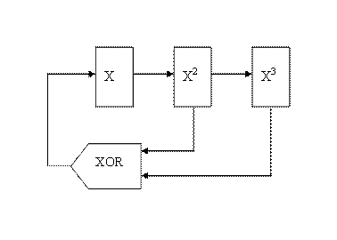
fig. 1
Because the operation of the register is deterministic, the sequence of values produced by the register is completely determined by its initial state (seed). Likewise, because the register has a finite number of possible states, it must eventually fall into a repeating cycle. However, PRNG with a well-chosen feedback function can produce a sequence of bits which appears to be a random one and has a very long cycle. The length of the maximum period doubles with each bit of added memory. It is easy to build PRNGs with periods so long that no classical computer could complete one cycle in the expected lifetime of the universe.
Nevertheless, the outputs of pseudorandom number generators are not
genuinely
random
—they only approximate some of the properties of random numbers.
John von Neumann
emphasized this circumstance with the remark "Anyone who considers
arithmetical methods of producing random digits is, of course, in a state of
sin”
So cryptography palters with facts contending that it is impossible to distinguish a PRNG sequences from the noise.
How to build a PRNG, satisfying the strictest cryptographic requirements? It is clear, that such a PRNG must occupy all the states of our World. Only in that case, owing to Physical incompleteness, we would not observe cycling in sequence of generating numbers. So if our Universe, as a whole, constitutes a big PRNG, then it will generate genuinely random numbers, as it apparently takes place in our real world. Indeed, when a quantum system passes to a definite single state, we can speak only of probability. And we can't predict beforehand what a hall the electron will prefer in consequence of measuring. So, we have illustrated that the world is deterministic for an objective observer and can be indeterministic for a subjective observer.
4. Geometry of (3,1) – world.
4.1 Analogy between quantum measurement and mathematical theory of error correction codes
There is an interesting parallel between our model and the mathematical theory of error correction codes [12]. As mentioned above, due to physical incompleteness, every quantum state is made up of hidden states. That is, the physical state is a subset of fundamental states. In the same way a code of n length is a subset of all possible vectors in binary space, which has the peculiarity that every two of them differ in at least some fixed number of places d (the minimum code range). The essence of the redundant coding lies in our confidence that distinct messages are encoded into code words that stay far apart from each other (in the Hamming metric). Therefore, one will not be confused with the other even in case of there having been some errors. The model (3,1) – corresponds to (3,1) – linear perfect code. The peculiarity of perfect codes consists in their ability to form "balls" around code words out of neighboring vectors and these "balls" pack the binary space completely; without gaps and crossings.
In the case of the (3,1) – model, the world consists only of 2 binary "balls" with radius R=1.
As shown on the fig.2, the distance between two physical "balls" is 1 bit and the distance between two code words (centers of balls) is 3 (so this code can correct one error). It is easy to see that the process of quantum reduction of state vectors is similar to error correction. The function of SO’s mind in our interpretation consists in a correction of errors in the communication link between himself and the objective reality.
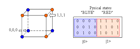
Fig. 2
PRNG generates some ergodic trajectory on this binary cube. So, half the time the system resides in the state |0> ("BLUE") and the other half in the state |1> ("RED"). The probability of finding the system for instance in physical state |0> (blue ball) at any definite moment of physical time is equal to ½.
The cycle period of this system is 8 algorithmic "seconds" which amounts to only 2 physical seconds. Therefore, each physical moment of time consists of 4 hidden algorithmic "seconds". In this hidden interval of time, the system can visit both physical states |1> and |2> and form a superposition. The space above the base of {|1>, |2>} in our example forms a two-dimensional Hilbert space of quantum states.
5. Quantum states and their superposition
We will now describe the world’s fundamental dynamics by utilization of an ergodic function ξ(τ) above the Galois field. Such a function can be set algorithmically, as described in section 3.
Let us introduce a predicate function:
![]() (3)
(3)
Which is equal to 1, if fundamental state ξ resides within the ball related to quantum state |x>, and 0 if not. We will show that the function:
![]() (4)
(4)
constitutes a quantum-similar state vector. Such construction allows us to define the probability of a physical state, as a square of absolute value of its state vector.
![]() (5)
(5)
Inverse elements in group multiplication are marked by an asterisk.
If for the same moment of physical time the system has sufficient algorithmic time to visit different physical states |0> and |1>, then we will say that a quantum-mechanical superposition [13] of these states takes place (Fig.3).
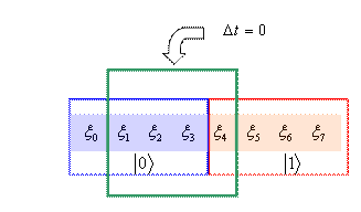
Fig. 3
Let us start by building the orthogonal functions Ф(τ,x) for the superposition, represented in fig 3.
![]() ;
;
![]() (6)
(6)
The state vector of this superposition is represented by the following construction:

Here we have truncated the normalization factor. The sense of this construction is very simple. If in the moment of the hidden time τ the system resides in |1>, then it can not reside at the same time in |0>. The functions ζ(τ,1) and ζ(τ,0) are orthogonal. Hence, we restore the status quo of Aristotelian logic at the fundamental level of the Universe. At a more "rough" level, meaning the physical reality level, the apparent violation of this logic occurs. Indeed, different physical (quantum) states for SO can exist simultaneously with different probabilities. It is easy to see that the probabilities for the base states are:
<x1|x1>=1/4 ; <x2|x2>=3/4 (8)
And the probabilities for transition from the state of superposition to the base states are:
<x1|x12>=1/4 и <x2|x12>=3/4 (9)
6. Operators in objective representation
6.1 observables
Let us write down what is observable for the quantum states {|1>, |2>}, considered above. In the representation of its own eigenstates it will look like:
 ; (10)
Such operators, applied often in KM we call - operators of the subjective observer.
By means of the operator (10), it is easy to find the expectation value of the measured parameter:
 (11)
(11)
We will now introduce the operator of an objective observer. In objective
representation, the sense of this formalism gets an obvious look: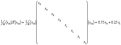 (12)
(12)
Unlike the ordinary KM, the operator in (12) works in the base of the objective observer.
Values of probabilities in (12) are caused by the simple circumstance that, according to (7), our system visits |2> three times more often then |1> in the process of algorithmic evolution.
6.2 Evolution Operators
In the same way, as shown above, we introduce the unitary operator of objective evolution.
It can be written as:
 (13)
(13)
This operator shifts cyclical components of the |x> vector. Recurrence equation of evolution is shown below:
![]() (14)
(14)
This equation describes the dynamics of vector |x> in ordinary physical time. As time flows, the vector turns in Hilbert space.
It is necessary to pay a special attention to the operators:
![]() и
и
![]() (15)
(15)
The operator Uπ is used as logical gate NOT in quantum calculations
[14]. Operator Uπ/2 executes the
operation![]() ,
which translates q-bits in superposition state.
,
which translates q-bits in superposition state.
Here, one should not focus on the formal side of the description, but to its physical sense, which escapes our comprehension in the case of an ordinary QM description.
Let us consider first the mechanism of action of the Uπ=NOT operator. This operator shifts cyclic components of vector (7) for 4 steps.
Obviously,
after a single application of Uπ to system in
![]() state, it turns to
state, it turns to
![]() , and vice versa. In other words, regardless of the
algorithmic
, and vice versa. In other words, regardless of the
algorithmic
state, we have inversion of the current physical state with probability 1.
The mechanism of action of operator Uπ/2 consists in cyclic shift of vector (7) for 2 steps. It is clear that after one application of Uπ/2 we will arrive to the system in its previous state or its opposite state with a fifty-fifty probability. The measured result depends on the initial algorithmic state (not accessible for SO) of the system. This viewpoint enables us to understand the origin of probabilistic character of quantum-mechanical measuring.
7. Conclusion
In this paper, we discussed the origins of quantum physics. We have introduced a new class of Quasi-classical finite-state models. The peculiar properties of these models consist of the abandonment from the objective character of the laws of nature. We have endeavored to answer the following question: what our artificial world looks like from the subjective point of view of an observer within the artificial world? Prior to our attempt to answer this question, we have constructed a model of the observer and placed it in this finite world. This approach enables us to show the quantum-similar character of the laws, generated by a model of this kind. Moreover, within this structure we have found the explanation of quantum non-locality. Physical incompleteness leads us to the concept of hidden time. We have showed that several instants of time coexist in the same moment in the manner suggested by Bohm [15]. Therefore, we must conclude that quantum laws of the real world may be understood from exactly such a procedure.
References
1.Stephen Wolfram A New Kind of Science Wolfram Media, Inc., 2002 ISBN 1-57955-008-8
2. Kurt Godel, "Uber formal unentscheidbare Satze der Pincipia Mathematica und
verwandter Systeme I", Monatshefte fur Mathematik und Physik, 38, 173-198, 1931.
3. Kaminski A. Physics simulation in the conditions of incompleteness. Quantum Magic v1. p. 3126-3149, 2004 http://quantmagic.narod.ru/volumes/VOL132004/p3126.pdf
4. Kurakin P. Hidden Time at Work: Simple Interference, Delayed Choice, Entanglement arXiv physics/0507142 http://arxiv.org/abs/physics/0507142
5. Xiaodong Chen "A New Interpretation of Quantum Theory. Time as Hidden Variable". Department of Physics, University of Utah, Salt Lake City, UT 84112 (March 29, 2000)
6. Kaminski A. The hidden space-time is in physics. Quantum Magic v2, p. 1101-1125 , 2005 http://www.quantmagic.narod.ru/volumes/VOL212005/p1101.pdf
7. John G. Cramer. The Transactional Interpretation of Quantum Mechanics Reviews of Modern Physics 58, 647-688, July (1986). http://mist.npl.washington.edu/npl/int_rep/tiqm/TI_toc.html
8. L.E. Dickson, American Mathematical Monthly, 1911, vol. 18, p.109. http://en.wikipedia.org/wiki/Finite_field
9. Felix M. Lev. Why is quantum physics based on complex numbers? arXiv:hep-th/0309003 v1. 29 Aug 2003 http://arxiv.org/pdf/hep-th/0309003
10. [6] H.B. Coish, Phys. Rev. 114, 383 (1959); I.S. Shapiro, Nucl. Phys.
21, 474 (1960);
11. From Wikipedia, the free encyclopedia.
http://en.wikipedia.org/wiki/Linear_feedback_shift_register
12. Berlekamp, E., Algebraic Coding Theory, McGraw-Hill, New York, 1968.
13. D. Bohm, Quantum Theory (Constable, London, England, 1954).
14. B. Hayes, “Computing Science: The Square Root of NOT,” American Scientist
83:4, 304–308 (1995).
15. D. Bohm, (1986), Time, The Implicate Order, And Pre-Space, in Physics and
the Ultimate Significance of Time, Ed., D. R. Griffin, 177-208, SUNY Press,
Albany.
![]()
![]()